Thursday, December 10, 2015

Lab 8 - Spectral Signature Analysis

Introduction:
The main objective of this lab was to gain an understanding of spectral signatures through collecting and analyzing them. To do so, 12 spectral signatures were collected of different surface features and analyzed by creating AOIs with the help of ERDAS 2013 polygon tool.

Methods:

The image used to gather spectral signatures was from 2000 specifically focusing on the Eau Claire and Chippewa Falls area, WI (Figure 1).
Figure 1 - Study Area


The 12 surfaces collected included:
1.  Standing Water
2.  Moving Water
3.  Vegetation
4.  Riparian Vegetation
5.  Crops
6.  Urban Grass
7.  Dry Soil (uncultivated)
8.  Moist Soil (uncultivated)
9.  Rock
10.  Asphalt Highway
11.  Airport Runway
12.  Concrete Surface (Parking lot)

Gathering spectral signature data using ERDAS is relatively simple. Under the drawing menu there is a polygon tool. (Figure 2)
Figure 2 - Polygon Tool icon

Using the polygon tool, a shape can be drawn on the image, creating an AOI or area of interest. Once the polygon is made, under the raster menu lies "Supervised" (Figure 3).
Figure 3 - Supervised

Under "Supervised" select "Create New Signature from AOI" and "Display Mean Plot Window". This adds the signature from the polygon to the new window and display the signature in graph form. (Figure 4)

Figure 4 - AOI with Plot


This step was done for each of the 12 surfaces. Some of the surfaces were hard to distinguish by just using the image from 2000. In that case, a linked Google Earth view was used to verify the surface was in fact the targeted surface. Once each of the 12 surfaces was collected they could be compared using the "Signature Mean Plot".  Signatures can be compared on the fly such as soil type signatures (Figure 5).
Figure 5 - Soil Signatures comapred

Results:

Looking at all 12 surfaces (Figure 6) we can see a wide variety in spectral signatures. This is due to factors such as moisture content, materials found in the surface, ect.

Figure 6 - 12 Surface Results

Sources: Wilson, Cyril. (2015). Geog 338: Remote Sensing of the Environment Lab 8 Spectral Signature Analysis. Personal collection of  Cyril Wilson, University of Wisconsin-Eau Claire, Eau Claire, Wisconsin.


Thursday, December 3, 2015

Lab 7 - Photogrammetry

Introduction:
With this lab the main focus is learning how to perform photogrammetric correction and manipulation using aerial photographs and also satellite imagery. Before diving in to the software and having ERDAS do the calculations it was import to understand the basic formulas and math behind the correction.

Methods:
As mentioned it is important to understand some basic calculations for measuring data on imagery. The first task was calculating the scale of a near vertical image. There is a number of methods that can be used to do the same task, it all depends on what data is presented and from there picking the method that best fits the scenario is the way to go.

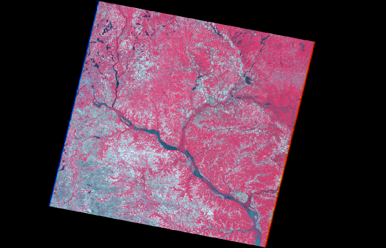
The first method for calculating scale is using an image (Figure 1) and picking two points on the image. The distance between these points can be compared to real world distance and be extrapolated from there. In the case of (Figure 1) the distance between A and B is 2.7 inches. The real world distance from A to B was 8822.47 ft. From there the next step is converting the real world distance to inches. The real world distance in inches is 105896.64. Because A to B on our image is 2.7 inches the fraction would be 2.7/105896.64 = 1/39210. With scale you want to round to the nearest whole number so in this case the scale is 1/40,000.
Figure 1 - Image with Point A and B


If you don't have the real world distance that doesn't mean you are out of luck it simply means you have to depend on using other methods. If the focal length of the camera is known along with the height the image was taken at it is still possible to calculate the scale. For the purpose of this image (Figure 2) the image was taken at a height of 20,000 ft and the camera it was taken with had a focal length of 152 mm. The ground elevation for the study area was 769ft.With all of this information known the first step is unit conversion. 152mm=.4986816ft. Now that the information is all in the same unit, inputting the information in to the formula Scale=f/H-h. .4986816/(20000-796) = .4986816/19204 = 1/38509. Once again it is important to round so the scale of this image is yet again, 1/40,000.
Figure 2 - Image used for calculating scale


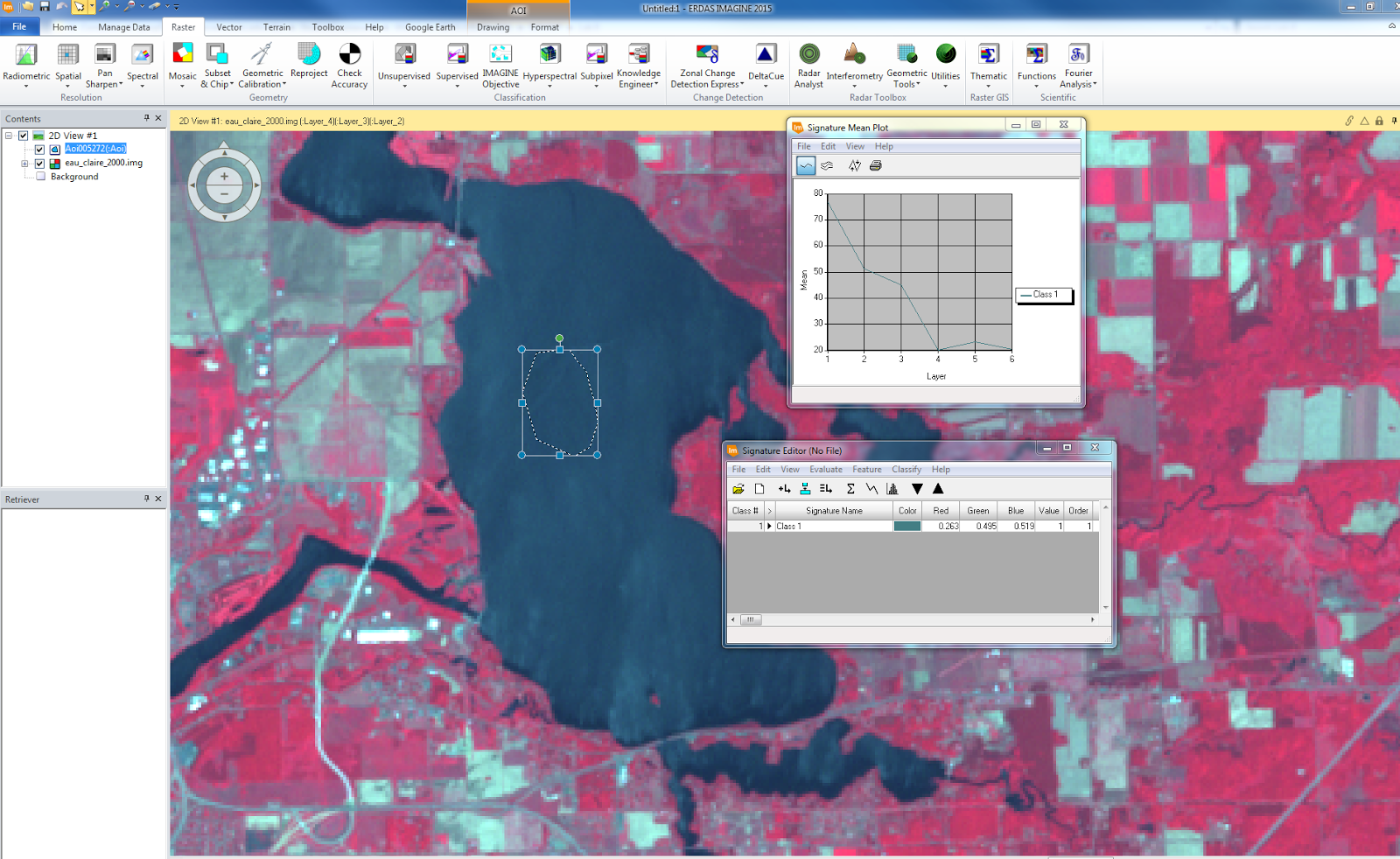
With the help of ERDAS, entire features can be measured on aerial photographs. ERDAS has a feature specifically for this called the Polygon Measurement Tool. This tool allows for users to draw polygons around a feature in order to gather data such as perimeter and area. In this image (Figure 3) a polygon was drawn around the lagoon and ERDAS presented the measurement data below in the measurements window. A number of units can be selected and changed on the fly depending on the unit of measurement needed for the project.
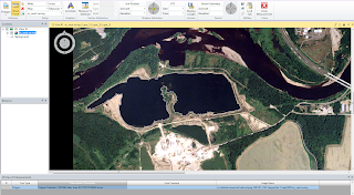
Figure 3 - Polygon with measurements below


Another aspect to consider when looking and analyzing aerial images is relief displacement. Relief displacement is essentially the variance of an object on an image from its true position on the ground. In (Figure 4) the smokestack featured appears to be leaning and not straight up and down when in actuality the smokestack is perpendicular from the ground. To calculate the displacement the variables needed are real world height, radial distance from principal point to the top of the displaced object and height of the camera. Displacement=h*r/H. The smokestack was 1604.5 inches and the radial dst was 10.5 inches. The camera height was 47760 inches. 1604.5*10.5/47760 = .352748. This means the smokestack needed to be moved .35248 inches to be vertical as it would be if you were at the base looking up at it.
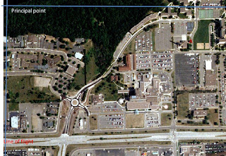
Figure 4 - Relief Displacement


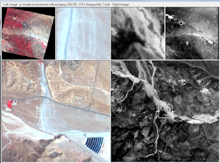
The next concept we touched on was stereoscopy which is using your eyes depth perception to view a 2D image in 3D. A number of tools can be used in ERDAS to accomplish this included the Stereoscope tool, anaglyph tool and with the assistance of red and blue "3D" polaroid glasses. Under the terrain menu in ERDAS the anaglyph tool can be found, after inserting the aerial image and DEM for an area (Figure 5) the tool can be used for creating an anaglyph image in ERDAS (Figure 6). With the assistance of glasses you can see that the elevation differences can be seen in 3D.

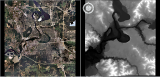
Figure 5 - Aerial Image and DEM
Figure 6 - Anaglyph created using Aerial Image and DEM

The last area of photogrammetry we focused on was orthorectification. Orthorectification is used to removed errors regarding position and elevation from gathering points on various forms of imagery. To do so accurately, not only x and y data has to be found and used but also z or elevation. To orthorectify ERDAS has a tool called Imagine Photogrammetric Suite. This tool can be used for a variety of purposes including orthorectification and triangulation. The goal of this section of the lab was to use a series of images and orthorectify them to create an accurate orthoimage. The images used overlapped but not evenly at the same point and needed to be corrected.

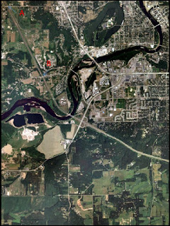
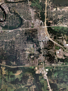
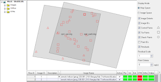
The first step was to open up Image Photogrammetry Project Manager and create a new block file. For this project the Geometric Model Category was set to Polynomial-based Pushbroom and also SPOT Pushbroom. Under Block Proptery Setup the projection was set to UTM - Clarke 1866 and the Datum to NAD 27 - (CONUS). After these settings were selected the first image could be brought in. The next step was to begin collecting GCP's. A reference image was brought in and 9 GCP locations were selected (Figure 7) with some guidance from Dr. Wilson.  2 additional GCPs were gathered from another reference image. After all the GCPs were selected the table contained x and y values but lacked elevation. The z values were filled in using data automatically inputted from the DEM. Once gathering all the x,y and z points were gathered the second image could be added to be corrected. For this to be done the Type and Usage for the control points had to be changed to Full and Control respectively.


Figure 7 - Adding GCPs


Using a similar method I was able to add the 11 GCP points from the first image to the second. This was a rather quick process.

Once correlating all 11 GCPs the Automatic Tie Point Generator could be used to calculate and find tie points between the tow images. This was done through a process called block triangulation, for a successful block triangulation at least 9 tie points are required. When setting up the Automatic Tie Point Generator the settings used were Image Used - All Available and Initial Type - Exterior/Header/GCP. The number of points I desired was set to 40. After the tool finished running I inspected the summary and looked at the tie points to verify the tie points found were accurate.

One of the last steps required was running the Triangulation tool. After the tool finished running, a report was created displaying the accuracy levels (Figure 8).
Figure 8 - Triangulated Images


The final step was running the Ortho Resampling too. Using the first image and the DEM with the settings selecting Resampling Method - Bilinear Interpolation, along with the second imaged added to tool was ready to be run.


Results:

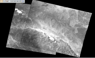
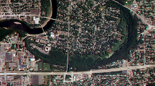
Figure 9 - Orthorectified Results


The results above (Figure 9) show a Orthorectified image that is accurately corrected. The only difference between the two images is a slight color change where the images are fused but hardly noticeable.

Source:
Wilson, Cyril. (2015). Geog 338: Remote Sensing of the Environment Lab 7 Photogrammetry. 
 Cyril Wilson, University of Wisconsin-Eau Claire, Eau Claire, Wisconsin.
ERDAS Imagine

Thursday, November 19, 2015

Lab 6 - Geometric Correction

Introduction
     Lab 6 focused on a form of image processing technique known as geometric correction and the various ways of accomplishing it. This lab focused on two specific techniques. Those two types of correction are known as image-to-map rectification and image-to-image. These are both done to help ensure image accuracy before it is interpreted and processed.

Methods

The first form of correction we focused on was image-to-map rectification. The goal of this part of the lab was to take an image that was inaccurate and correct it using a map. Hence the name image-to-map rectification. Our study area was Chicago. In order to correct the image, the user must use Ground Control Points or GCPs. GCPs are points the user puts on both the image and the map. They should be as close as possible to the same location on both the image and map. Depending on the image delegates how many points will be needed to correct it. In the case of our image, there was low distortion meaning it was a first order polynomial. Going off this chart (Figure 1) a minimum of 3 GCPs are required.
Figure 1 - Required amount of GCPs
While adding GCPs it is important to check the level of accuracy you are achieving. Erdas Imagine has a feature that monitors the Root Mean Square or RMS while adding points. For any image you want to shoot for under 2.0 RMS (Figure 2) but the ideal level is less than .5.
Figure 2 - Adding GCPs and checking RMS error


Once satisfied with the level of accuracy it is time to re-sample the image. Re-sampling is mainly done to correct pixels that lack a brightness value. The final comparison of the first image vs. the corrected image can be found below (Figure 3).
Figure 3 - Resampled and corrected image overtop original
The second form of image correction we  did is referred to as image-to-image rectification. It is essentially the same process before except instead of a map we are using another image that is spatially accurate. Our study area for this correction is Sierra Leone. This image (Figure 4) happened to be a lot more distorted than the Chicago image and requires a third order polynomial. If we check the chart (Figure 1) we can see that at least 10 GCPs have to be used. After placing the GCPs (12) of them I got my RMS error to be less than 1 (Figure 5)

Figure 4 - Spliced Image presenting the differences between the distorted image and the already corrected image


Figure 5 - GCPs placed on image and RMS error lowered

Once again, after completion the corrected image had to be re-sampled. Because bilinear interpolation is more accurate I re-sampled using that method instead of nearest neighbor and the results were accurate and smooth (Figure 6)
Figure 6 - Finished image spliced with original corrected image
Conclusion
Images that are properly geometrically corrected and very important when doing accurate analysis. GCP location is essential for obtaining the highest accuracy and getting the RMS error the lowest possible should be a priority. Tools like ERDAS make correction relatively easy if you know the correct methods and what re-sample method to use.

Sources -
Images - U.S. Geologic Survey
Program Used - ERDAS Image

Thursday, November 12, 2015

Lab 5 - Introduction to LIDAR

Background and Goals

This lab's main purpose was introducing us to Lidar and how it can be processed and manipulated. Lidar is a form of active remote sensing. Basically Lidar works by sending a laser pulse to the ground from an aircraft, the pulse then returns to a sensor mounted on the aircraft. This data is used to create a point cloud. This data is separated in to different return heights allowing to calculate location and elevation.

This lab was meant to introduce us to Lidar while showing us the basics in an area we are familiar with, Eau Claire, Wisconsin.

Methods

The very first step of the lab was to import the Lidar data in to a program that would help us view the data. For this lab we once again used, Erdas Imagine. Erdas Imagine has a lot of visual tools to view LAS point cloud files.

We also used ArcMap for the majority of the lab because it allows us to examine the statistical data of the imagery. While looking at the elevation statistics it shows that our study area (Eau Claire) is around 1000ft while there was one value around 1800ft. (Figure 1) The Z value represents elevation.  ( Later in the lab while exploring the data I found out what was responsible for the anomaly.
Figure 1 - Table showing Z Max & Mins

Often times Lidar data lacks a coordinate system so the user must define one while examining the metadata. (Figure 2)
Figure 2 - Coordinate Systems Specifications
By looking at the metadata we can tell that our XY coordinate system needs to be NAD 1983 and our Y coordinate system should be NAD1988. To adjust these coordinate systems you have to go under the LAS Dataset Properties.

With the LAS Dataset Toolbar enabled a user can look at the surface data in a number of ways included Elevation, Aspect, Slope, Contour. I predominantly used Elevation but it varies depending on what you are doing with the data.

Occasionally there are missing chunks of data. In our dataset one instance of that was in a chunk of water. Without having the data Arc could not determines a value so the program guessed and made it seem like there was elevated water there when in actuality, data was just missing. (Figure 3)
Figure 3 - Missing water data
Like mentioned earlier, when "touring" the data I came across a very specific "high point" in elevation. When looking at it in 3D view it became more apparent of what the high spike in elevation was. (Figure 4)
Figure 4 - 1800ft Tower

The point in data stood out so vividly because as you can see everything surrounding it is much, much shorter. This appears to be some sort of radio/television tower. The 1800ft elevation makes much more sense now knowing this can be found in Eau Claire.

Using ArcMap tools, Lidar data can be turned in to 3D images. For example, we took the first return data for Eau Claire and created a digital surface model (DSM) (Figure 5) at a resolution set at 2 meters. We also made a digital terrain model (DTM) (Figure 7). Lastly, a hillshade model was created to enhance the DSM. (Figure 6)

To do this the LAS Dataset to Raster tool was used with the Value Field set to Elevation, Cell Type: Maximum and Void Filling: Natural Neighbors. In addition, the Cell Size was set to 6.56168 which equates to basically 2 meters.
Figure 5 - DSM

Figure 6 - DSM with Hillshade


Figure 7 - DTM of study area


 To create the DTM you have to set the filter to "Ground" this creates a "bare earth" raster image. This eliminates buildings and trees and focuses on terrain and elevation.

The last iteration of the data I created was an "Intensity" image. This is created using first return data. Once again using the LAS Dataset to Raster tool. The only thing changed settings wise is Value Field which has requires Intensity to be selected. The produced image was dark, not showing great detail but once lightened in ArcMap the image was enhanced and very detailed. (Figure 8)

Figure 8 - Intensity image created and brightened in ArcMap
Result
This lab lays out the basics of Lidar and highlights a few ways the data can be used for image processing. Lidar is an ever expanding field and I only expect it to become more popular and easier to work with. ArcMap and Erdas compliment each other very well when working with Lidar and I look forward to digging further in to Lidar.

Sources:
Lidar point cloud and Tile Index obtained from Eau Claire County, 2013.
Eau Claire County Shapefile is from Mastering ArcGIS 6th Edition data by Margaret Price, 2014.

Thursday, October 29, 2015

Lab 4 - Misc. Image Functions

Goal and Background:
Images we are presented with may not be perfect or ideal all the time. Fortunately for us there are several methods too correct and fix images to make them clear and usable. In this lab I will be focusing on techniques such as creating a subset, haze reduction and image fusion.

Methods

Image Subsetting
Creating a subset is pretty straightforward and easy to do with the tool Erdas Imagine provides. Like with most things there are many methods of accomplishing this but the easiest method is to open up you image and insert an inquire box. Place the box over the area you want to focus and from there click "create subset" from the above menu. From here save the subset under any name you want and you now have your subset or area of interest.

 
Original Satellite Image
 
 
Subset from Original Image
This is an important tool because often satellite images cover a massive amount of land space when in actuality you really only desire to work with a small portion. Subsetting an image focuses on a smaller area that is more useable and easier to interpret.

Image Fusion
The main reason you would want to use image fusion is for enhancing the quality of an image by combining it with another image. This is referred to as pan sharpening. To achieve higher quality means taking a reflective and panchromatic and fusing them together thus creating a pan sharpened image. In this case the reflective image has a spatial resolution of 30m and the panchromatic is 15m. When combining the two the image takes on the smaller pixel size, showing more detail. At full extent you may not see a difference in image quality unless you zoom in. The image quality does not get distorted as soon, showing greater detail.


Pan Sharpened Image
Haze Reduction
Unfortunately haze is a factor we have to contribute while dealing with imagery. Fortunately, there are ways of reducing the significance haze has on an image. The more haze an image has the harder it is to interpret accurately and efficiently. ERDAS has a tool specifically made for reducing haze in an image and it works surprisingly well.  
 
Image featuring haze in the southern most part

Image after haze reduction - notice the slight change in color and improvement
Linking Erdas with Google Earth
Sometimes when interpreting an image you may come across something you simply cannot decipher with the given image. Syncing your image up with Google Earth may assist you because Google Earth supplies us with very high quality images in true color. This means you are able to zoom in very far without distortion and can use Google Earth as a reference point and decipher the image you have using clues from the usually up to date Google Earth imagery.

Erdas Image and Google Earth Synced

Resampling
Resample is used in instances where you want to increase or decrease pixel size of an image. This is particularly important when needing to interpret images. When increasing the pixel size it is referred to as resampling down while decreasing the pixel size is resampling up. With your image in the viewer go to spatial options and from there you can use the tool to adjust the pixel size by simply typing in the new desired dimensions.
This image has been resampled from 30mX30m to 20mX20m
Mosaicking
Mosaicking is a needed tool when your study area is larger than a given satellite image or split between two. Erdas has two forms of mosaicking, Mosaic Express which is very fast and easy and Mosaic Pro which creates more detailed, seamless mosaics but takes a little longer and is not as user friendly. With Mosaic Express you can tell there is more than one image being used based on color alone. The images do not blend well together although lined up correctly. Mosaic Pro, blends the colors and makes for a seamless mosaic of two images.
Mosaic Express Image


Mosaic Pro Image

Binary Change Detection / Image Differencing
Image differencing is simply comparing two images and finding the differences between the two images. In our case we looked at images of the same location 20 years apart. In Erdas there is a model builder that you can create a model to achieve certain goals. In this case I created a model comparing the two images specifically looking for loss of brightness in pixels. I also created a model that looked for pixels that did not change between the two images. Once combining those two files and putting them in to ArcGIS you can create a map showing changes between the two pictures.


Results
When working with images you often come across what some may consider problems or issues but with programs such as Erdas and the tools they have, working on these problems and fixing them is relatively easy as you can see from all the examples above.
 
Sources:
Cyril Wilson - UWEC - Fall 2015
ERDAS Image
Google Earth
ArcGIS